About paper
Czech originalHow to draw 2D oscillations and Lissajous curves using 3D projection
Abstract
This contribution presents possibilities of dynamic modelling that was developed using PHP for composition of perpendicular commensurable oscillations in plane. Modelling is accompanied by a real 3D model realized on a transparent foil with whose 2D projection one can verify the results with students.
Introduction
There is no need to repeat that computer technology has already become a regularly used didactic technology and we meet it in education at all school levels. However, less often we use its capabilities to prepare sources for construction of real teaching aids at school.
When we focus on dynamic simulations in physics, mainly in the basic physics course, we can advantageously use not only special programmes but we can also prepare our own models on the basis of freely accessible platforms.
When making dynamic models we most often meet those in which some quantity changes in time. Such simulations are the most suitable ones to replace the usual way of showing just a result of an analytic solution when the solving itself and the calculation of which is beyond the limited education time frame or eventually beyond the abilities of students as we have noted in our previous paper [5].
Composition of perpendicular oscillations
The graphic result of the composition of two mutually perpendicular oscillations in a plane is one of the Lissajous curves that are used to compare the frequencies and phases of two oscillations. If the ratio of their frequencies is a rational number (1:2, 2:3, 5:7, …), the corresponding Lissajous curve is closed and is clearly observable. In other words, the movement of a real body or a point that oscillates in two perpendicular directions at such two frequencies is periodic.
The individual oscillations on axis X and Y can be described as:
\[ x = X_0 \sin(\omega_x t + \varphi_x), \] \[ y = Y_0 \sin(\omega_y t + \varphi_y). \]By subtracting initial phases of these oscillations we get their mutual phase shift:
\[ \varphi = \varphi_x - \varphi_y .\]If the phase shift is zero, we get the basic shape of the curve. The process of manual calculation of the above mentioned equations would be very lengthy. For this reason we can have these curves (see Fig. 1 and 2) generated by a computer.
We may ask the following question when we construct the Lissajous curves:
“Does the generated pattern change when we change the phases of oscillations at given frequencies fx, fy?”
Dynamic modelling helps us to find the answer.
When we practise composition of perpendicular oscillations with an oscilloscope in laboratory classes and we try to create a Lissajous curve, we can observe the following effect: When the time base (Volt/point) is not set properly, the pattern is moving on the screen of the oscilloscope as if it was rotating. Upon detailed observation we realize that the way we interpret Lissajous curves in 2D is not a complete piece of information. We can imagine the pattern itself as if it was drawn around the surface of a transparent cylinder and we just moved around this cylinder and changed our observation angle. We can see the pattern both on the near and on the far surface because the cylinder is transparent. The pattern that is created by simultaneous back and front projection is thence not always new; it is only seen from a different angle.
It must be noted that this movement of the observation point around the cylinder does not have to be evident at a glance because the more distant part of the curve is not smaller. We miss the perspective and are naturally confused.
Results of modelling of perpendicular oscillations in PHP
Results of PHP modelling of perpendicular oscillations with frequencies in the ratio 1:1 and 2:3 are displayed for different phase shifts in Figures 1 and 2 respectively (see [4] for further reference).
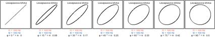
Fig. 1 Lissajous curves for frequency ratio 1:1 with phase shift increasing by 15°
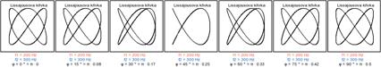
Fig. 2 Lissajous curves for frequency ratio 2:3 with phase shift increasing by 15°
3D-aid for creating Lissajous curves
Lissajous curves can also be demonstrated using a Blackburn pendulum or wound transparent foils. Demonstration with foils is simpler and needs less time for preparation. We printed the patterns shown in Fig. 3 on transparent foils to demonstrate curves with frequency ratio 1:1, 2:1 and 2:3. Then we wound and glued the ends of each foil together.
![]()
Fig. 3 Figures for demonstration of Lissajous curves with frequency ratios 1:1, 2:1 and 2:3
Photos in Figures 4 – 8 show Lissajous curves for different frequency ratios and phase shifts.
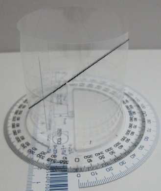
Fig. 4 Lissajous curve for frequency ratio 1:1 and 0° phase shift
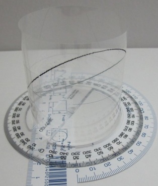
Fig. 5 Lissajous curve for frequency ratio 1:1 and 30° phase shift
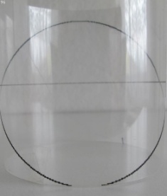
Fig. 6 Lissajous curve for frequency ratio 1:1 and 90° phase shift
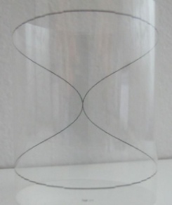
Fig. 7 Lissajous curve for frequency ratio 2:1
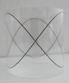
Fig. 8 Lissajous curve for frequency ratio 2:3
Conclusions
Dynamic modelling, not only in PHP, helps to create, use and deepen inter-subject relations and to go through the whole process of discovering and getting to know the laws of the nature. A precondition for this is a suitable coordination of teaching and curriculum in subjects between which we form these relations. “Point by point” drawing is usually used for showing the development of a dependence of two quantities.
On the example of composition of two oscillations we have shown that another suitable platform for dynamic modelling is PHP. It is very favourable when we can supplement a mathematical model with a really existing model that strongly helps to create an idea of the investigated process.
The Google Chart Tools application, which is a tool for creating graphs, equations and other graphical outputs, could also be a supplement to PHP modelling.
All the above mentioned methods were verified in practical education and benefits in better understanding of how the world “works” were achieved in comparison with a control group.
For the future we are preparing at least a partial introduction of interactivity in the models that we have been successively presenting at http://www.ped.muni.cz/modely and also alternatively at http://www.valek.pro/kmity .
Literatura
[1] BUREL, D. Úvod do práce s knihovnou GD v PHP [online]. 2008 [cit. 2009-11-23]. Available on the Internet:
<http://programujte.com/?akce=clanek&cl=2008010402-uvod-do-prace-s-knihovnou-gd-v-php>. ISSN 1801-1586.
[2] LEPIL, O., RICHTEREK, L. Dynamické modelování. Olomouc : Repronis, 2007. 160 s. ISBN 978-80-7329-156-3.
[3] ŠEDIVÝ, P. Modelování pohybů numerickými metodami : Studijní text pro řešitele FO č. 38. Hradec Králové. 1999. 38 s.
[4] VÁLEK, J., SLÁDEK, P.: Dynamické modelování kmitů [online]. 2010 [cit. 2011-08-08]. Available on the Internet: <http://www.ped.muni.cz/modely>.
[5] VÁLEK, J. Dynamické modelování v PHP. Veletrh nápadů učitelů fyziky 15. Praha : Prometheus, 2010. od s. 239-243, 5 s. ISBN 978-80-7196-417-9.