About paper
Czech originalExperiments in Malá Hraštice – this time with heat
This contribution describes:
1) simple demonstrations of adiabatic processes, showing the difference between adiabatic and isothermal processes, with the possibility to determine approximately the value of the Poisson constant \(\kappa = \frac{C_p}{C_V} \).
2) a group of experiments for the demonstration and measurement of heat transfer by radiation both by means of ICT (“datalogger”) and simple teaching aids that cost only a few crowns.
Introduction – What happens in Malá Hraštice
Spring trainings for future physics teachers and “soul mates” have been happening since 1997. Traditionally, we arrange it in a camp near the small village of Malá Hraštice not far from Dobříš at the beginning of May. The trainings last 4-5 days and there are 15-25 participants.
Mostly, there are students from the physics education department from our faculty including PhD students, but many others who teach at schools and other guests come here too.
The training is very informal and completely voluntary. Students do not get any credits or anything else for participation. We go to Hraštice to have fun with physics. Moreover, (as man does not live by physics alone), there is also a non-scientific program. The scientific part of the program is mostly realised in the form of miniprojects. Duos, trios or any other groups of participants choose themes in which they are interested and they try to fathom something. Naturally, it is not about discovering “new physics”, but it is about trying some experiment, devising a new variant or trying to measure something. Moreover, we do not do it in school or in a scientific laboratory, but literally in “field conditions” where we have to improvise, exploit simple materials and find out nonstandard solutions. It is obvious that it trains creativity, physical intuition and all sorts of skills. The results are then informally presented by participants. The results could be, as in real scientific research, negative findings like “there is no way”, “it is much more complicated than I thought”, and eventually “we have to look at it closer”.
Interested persons may find details of the trainings and miniprojects here [1]. I would like to mention one important aspect: the trainings make it possible to try many things and bring ideas and inspiration for new experiments or their variants and new simple devices and tools. Many of these themes that were developed or first tested in Malá Hraštice were already published in the memorial volume of the Veletrh nápadů [2], [3].
In 2008 the main theme of the scientific program was Heat. In the following text I will describe two examples of experiments that I tried there.
Adiabatic and isothermal processes in a simple and clear way
Isothermal and especially adiabatic processes are taught only theoretically in physics at secondary school. The following simple experiment makes it possible to demonstrate their difference – and moreover to approximately determine the value of the Poisson constant.
The principle of the experiment is shown in Figures 1 and 2 respectively. A tube containing a few centimetres water column passes through a bottle neck. There is air in the bottle. If the tube is oriented horizontally, there is atmospheric pressure in the bottle.

Fig. 1: If the tube is horizontally oriented, inside the bottle is the same pressure as in the surrounding atmosphere

Fig. 2: The pressure increases in a vertical orientation
If we turn the bottle with tube into a vertical orientation (see Figure 2), the pressure in the bottle increases because of the hydrostatic pressure that is given by the height of the water column. The air in the bottle is a little compressed and the column of water shifts down.
Where is the difference between the adiabatic and isothermal processes that I promised?
If we do an experiment, we will see.
At first the water column falls down rapidly, but then it falls slowly. The first fast falling down, that is connected with the compressing of air in the bottle, is a process that is very fast so that the air temperature in the bottle has no chance to achieve the same temperature as its surroundings. Therefore the process is same as if the air in the bottle was heat insulated – the process is adiabatic. During this process the pressure increases faster during compression than during an isothermal process. Therefore we need a smaller compression (a smaller decline of water) to keep the water column balanced by overpressure. Air in the bottle heats a little bit, but in this experiment we do not measure it or find it out.
In a few seconds the air temperature is equal to the surrounding temperature, therefore it is the same as at the beginning. Hence, we can use the equation for an isothermal process for the air volume in the bottle: p·V=const. Still, without calculation, only by physical intuition, it is obvious that if the air in the bottle cools down again, its volume decreases and the water column in the tube goes down.
Afew quantitative estimates and calculations
Let’s start with an isothermal process. From the equation pV = constant we can calculate the relation for volume change \(\Delta V \dot{=} - \left( \frac{V}{p}\right) \Delta p \) by derivation of the respective differential. However, we can calculate this only with university level knowledge of maths. Hence, let us try it more simply by asking students a question: If the pressure increases about 1 %, how much must the volume decrease to keep the product pV constant?
Surely, the volume must decrease also by about 1 %. (You can persuade students by dividing 1 by 1.01 or multiplying 1.01 by 0.99 or otherwise. It is good to point out to students, that this calculation is correct only for small changes of pressure. Naturally, with a 200 % increase of pressure the volume does not decrease about 200 %.)
The pressure increasing about 1 % equates to a 10 cm height of water column (Either we can calculate it from equation \(\Delta p = \Delta h \rho g \) or we can recall that 10 cm is a hundredth of 10 m, which is the height of a water column that is in equilibrium with atmospheric pressure). If the bottle has volume 0.5 l and the tube has an inner diameter of 4.4 mm (the area of the inner cross-section is about 0.15 cm2), a volume change of about 1% corresponds to a shift of the water column of about 33 cm. For a water column of height 5cm the pressure and volume change would be 0.5 %, the water column would decrease about 17 cm and so on.
What about adiabatic processes? Now the equation is \( p V^{\kappa} = const.\) An increase of pressure of about 1 % does not correspond to a decrease of volume of about 1 %, but only about 1/κ %. For κ = 1.4 the volume decreases about 0.7 %. We can simply calculate this effect: try to multiply 1.01 times 0.9931.4. Of course, in seminars with students who know calculus you can deduce the general equation \[ \Delta V \dot{=} - \left( \frac{V}{\kappa p}\right) \Delta p .\]
For the above-mentioned example (the halfliter bottle and tube with 4.4 mm diameter) the decrease due to a 1 % pressure increase is less than 24 cm, for a half-high column the decrease is also half.
The important thing is that the ratio of the length of the water column’s shift during an isothermal process (lI) and during an adiabatic process (lA) is equal to the Poisson constant κ.
\[ \frac{l_I}{l_A} = \kappa \]This can be seen both from the above example and from the general equation.
Realization of experiment
The experiment can be done with the simplest teaching aids. Instead of a glass tube we can use a hose made from plastic material that we can buy in gardener’s shops. Its inner diameter is 4.4 mm. The hose can be put on the tip of a plastic syringe. This 20 ml syringe with the end cut off can be tightly put into the neck of a plastic bottle. We stick a scale paper or ruler to the hose – now we can start the measurement. One bit of technical advice: when we change the position of the hose from horizontal to vertical it is good to stop the end of the hose with a finger. After this water column stays at its initial place, it starts to decrease, after we loosen the finger.
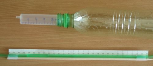
Fig. 3: Realization of experiment
Naturally, this measurement is fairly rough. The water in the hose has sometimes a tendency to get “stuck” (it is useful to tap on the hose), and moreover it is difficult to read accurately the position of the water column during the first rapid decrease (the value of lA) etc. However, the results do give the value of Poisson‘s constant near 1.4 (this is the tabulated value for air).
One other warning: do not take the plastic bottle in your hands during measurement. If the bottle warms up from the heat of your hands, the air inside expands and we have a „thermoscope“ instead of a device for k measurement.
Heat transfer by radiation
Lots of contributions were devoted to demonstrating heat transfer by radiation at VELETRH NAPADU. What about trying to quantitatively measure the radiation heat transfer – for instance from the Sun, but not only from it, with simple teaching aids and as quickly as possible.
The LabQuest system from the Vernier corporation (see [4]) with a small probe for measurement of temperature helps us in Hraštice. It is a small portable device for collection of computer data from experiment. Its advantage is that you can bring it with you to the country or you can use it in “field conditions” at trainings like Hraštice. This is exactly what we did. I stuck the probe for temperature measurement on a piece of copper plate (5x5 cm) with cellotape. This copper plate I sprayed with black varnish on one side. On the other side the copper plate was isolated by polystyrene (the polystyrene was attached to the plate while hot. It is possible to do this, if you heat the plate with a soldering iron – naturally before attaching the probe).
If the blackened plate is exposed to solar radiation, it heats up quickly. Labquest collects data (the default is every half second), it can plot the data in a Figure and fit the part of them with linear dependence – hence, we can calculate the temperature increase with time – see Figure 4.
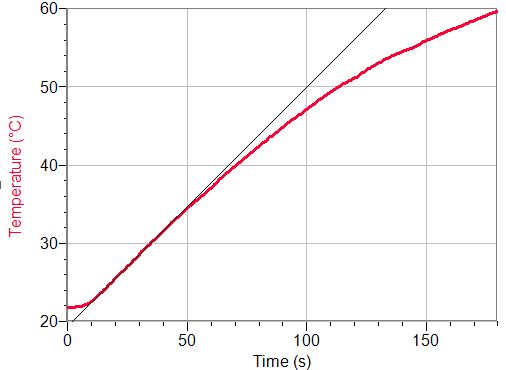
Fig. 4: The temperature increase of a blackened copper plate that is heated up by solar radiation
Naturally, at higher temperature the temperature increases more slowly (the plate is cooled down e.g. by the surrounding air), but at the beginning the temperature increases linearly – in our case at about 0.3-0.33 K.s-1. From the heat capacity of the plate (that we have determined from its mass and the specific heat capacity of copper) we can calculate that the plate was heated up by power of about 1.5 W. After recalculation to square meters we get 600 W.m-2. This value is lower than the solar constant (also lower than the intensity of solar radiation at theEarth’s surface that is about 1 kW.m-2) but they are of the same order. The difference can be explained by heat losses; furthermore the sky was not clear at all at the time of measurement.
We can heat up the blackened plate by other sources of radiation, for example:
· table lamp
· tin filled up with hot water (the tin has to be not shiny, so we spray it also with black colour)
· by one’s own palm. In this case the temperature increases more slowly – however it is only ten times slower than when we heat the plate by solar radiation. At the beginning the increase was about 0.03 K.s-1 (the length of palm in contact was 2 cm). If we use black aluminium sheeting instead of copper plate, the beginning rate of increase of temperature is 0.14 K.s-1.
How to measure a hundred times cheaper
The reader might be annoyed by the fact that previously I wrote about simple teaching aids and then the measurement was described using a LabQuest system that costs about 10 000 crowns. Let us see how to do this more cheaply with the help of a common multimeter.
If we have a multimeter with a probe for temperature measurement we can exploit it – of course the accuracy of the measurement is on the order of a degree. The second possibility is to use a bead thermistor (the price is around ten crowns) and to measure its resistivity by multimeter. However, we have to measure the temperature dependence before starting our measurement (i.e., we have to do a calibration). With the help of a battery and a few resistors we can use a multimeter to measure voltage and show that the data is increasing with temperature. Moreover, it approximately numerically matches the measured temperature. The details exceed the scope of this article – hopefully we will discuss it in the future.
References
[1] Dvořák L.: Labs outside labs: miniprojects at a spring camp for future physics teachers. European Journal of Physics 28 (2007), S95–S104.
[2] Dvořák L.: Trocha heuristiky z Malé Hraštici. In: Sborník konference Veletrh nápadů učitelů fyziky 5. Ed.: Rauner K., ZČU Plzeň 2001, s.143–146.
[3] Dvořák L.: Netradiční měřicí přístroje 4: Měření krátkých časů. In: Sborník konference Veletrh nápadů učitelů fyziky 9, svazek I, Ed. Smetanová J., Sládek P., Paido 2004, s. 30–32.
[4] Pazdera V.: LabQuest – měření v terénu. Příspěvek v tomto sborníku.