About paper
Czech originalPhysics on an Airplane
Abstract
We made an appointment with aerobatic pilots, fixed some cameras and Vernier sensors and probes on their airplane and on the pilots themselves and studied the course of an aerobatic flight.
Used Equipment
In addition to the airplane and the enthusiastic pilots capable of (almost) anything we used also:
• Vernier LabQuest 2 datalogger [1]
• 25-g Accelerometer [2]
• Barometer [3]
• wireless Exercise Heart Rate Monitor [4]
• Vernier Logger Pro software [5]
• a set of cameras some of which we attached on the wing, tail and inside the cockpit
What have we found out – proposals on activities with students
Stroboscopic effect
The stroboscopic effect can be nicely seen on the propeller in the recording of the start of the plane. First the propeller seems to rotate in one direction, then in a short while it stands still, and then it starts rotating in the other direction and the plane rushes forth.
Flexibility of wings, action of flaps
On the video recording from the wing of the plane we can notice that the whole airplane is in fact very flexible, the wings bend visibly during the flight. One can also watch the action of flaps during individual manoeuvres.
Accelerometer data
Vernier offers several different accelerometers: one‑dimensional accelerometer up to 5 g, three‑axis accelerometer up to 5 g, three‑axis accelerometer up to 2 g built in the LabQuest 2 datalogger and also an one‑dimensional accelerometer for high accelerations up to 25 g. Expecting large accelerations, we used the last one.
We placed the sensor so that it measured in the direction feet–head. This direction is the most important for pilots because the human body is most sensitive to acceleration in this direction. Too high values of accelerations can induce a loss of consciousness.
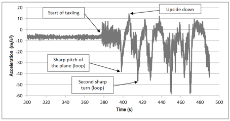
Fig. 1. The data from the accelerometer.
Figure 1 shows mild vibrations of the plane for the first 380 seconds approximately when it waits on the beginning of the runway and heats up the engine.
Attentive students may notice that the average value is not 10 m/s2 but less, approximately 7 m/s2. We can let them find the cause – it is because the pilot is not sitting straight in the plane. He is inclined with the seat and thus only a part of the gravitational acceleration is projected in the direction feet–head.
In the following 20 seconds (between 380 s and 400 s) the average value is about 7 m/s2 again but vibrations are much stronger because the plane is taking off.
Rapid changes of acceleration follow then during the aerobatic sequence. The first distinct local minimum corresponds to a rapid pitch of the plane (an altitude-gaining half loop) after which it ends upside down – the first notable local maximum corresponds to the final position. After that the pilot rolls the plane the right side up and flights so for 5 seconds during a horizontal section of the flight between 408 s and 413 s. Then another rapid loop follows etc.
Heart rate
The pilot had the heart rate sensor [4] fixed around his chest and the data was wirelessly transmitted to the LabQuest datalogger. From Figure 2 one can see that the heart rate rose during the flight and after landing it went down back to the initial value. It is interesting that one of the pilots had a rate of 140 beats/min (which corresponds to a quite intensive sport performance) while the other one had 110 beats/min. The latter is famous for his very calm temper which we assured ourselves.
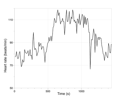
Fig. 2. Heart rate recording
Air pressure
We measured the air pressure with a barometer [4] placed inside the cockpit of the plane. GPS modules do not generally give very good information on altitude. The typical uncertainty is usually many times worse than with horizontal measurement which is given by unfavourable observation angle of individual satellites. For this reason we decided to measure changes of altitude with a barometer.
Because the air pressure changes quite fast with the weather, we made a correction on this change presuming a linear change of pressure during the ten-minute flight. Otherwise the pressure would have been different after landing and before take-off and it would have seemed from the pressure-altitude conversion that the plane landed a few meters above or below the ground.
We did no conversion on pressure change due to the air flow around the plane because we are not certain on how to precisely do it. The initial idea of using the Bernoulli equation turned out to be too optimistic. The result is that from the air pressure data it seems that the plane that was flying just above the ground (about 5 meters) is in an altitude of a few tens of meters. Because of this, we take the altitude data “less seriously” in the sense that they do not give the altitude with meter precision. Yet they can help us distinguish whether the plane flies straight or ascends or descends quickly.
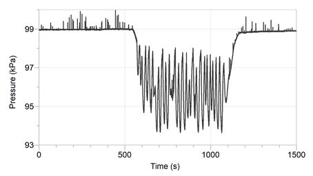
Fig. 3. Air pressure in the cockpit
The first part of Fig. 3 (up to approximately 600 seconds) responds to the plane waiting to take off. Then a ten-minute aerobatic sequence full of rapid changes of height follows and then the landing and stopping of the plane are captured in the graph.
Data from the GPS module
The GPS module that is integrated in the LabQuest 2 [1] datalogger was placed in the cockpit of the plane. Unfortunately any time the plane was upside down during the aerobatic flight, the GPS module could not “see the sky” and this became evident in the data by a jump in position.
Even though the GPS data are very interesting and can be nicely visualized in the programme Vernier Logger Pro [5]. Figure 4 nicely shows the trajectory of the plane above the airfield and its surroundings and also a beautiful huge arc before landing.
The programme Logger Pro enables also replaying of the data. Thus we can let the plots (trajectory, pressure, heart rate and so on) draw progressively in real time, in slow or in fast motion.
The data can also be exported to Google maps so that we can see the trajectory on the background of a real map. Previously (up to a certain phase of the year 2012) Google allowed to display in its maps a virtually unlimited amount of data such as ten thousands of entries of position, speed, instant noise, temperature etc. That enabled one to go through the landscape (or a city for example) and every second automatically measure relevant data and the position where they were taken using LabQuest – and then display the whole walk including measured data in a map. It seems that Google has changed its policy recently and currently it enables displaying of only a few hundreds of data entries in a map, which is sufficient for biologists for field measurements for example but is insufficient for the trajectory of a motion. We will keep on investigating this thing.
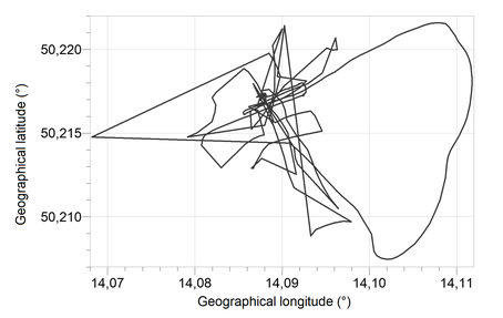
Fig. 4. 2D trajectory of the flight acquired by the GPS module in LabQuest 2
3D trajectory of the movement of the plane
Because we have the data (although with a certain error) on position (from the GPS) and on the altitude (from the barometer), we can put together also a three-dimensional model of the trajectory of the aerobatic flight.
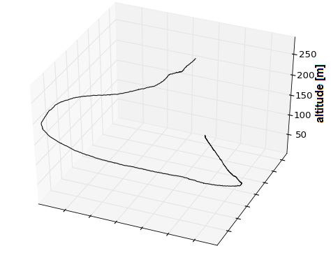
Fig. 5. Three-dimensional trajectory of the movement of the plane
Figure 5 shows an example of a 3D graph made in Python by David Roesel who is a student of the PORG Libeň Secondary School. In David’s programme the motion can be animated and the graph can be arbitrarily rotated. The last part of the flight with a huge arc around the airfield is displayed here.
Some interesting numbers
The speedup from 0 to 200 km/h during the start took only 20 s with an acceleration of 3 m/s2 and the total path taken was 650 m.
The maximum rate of ascending was 30 m/s.
The maximum G-force in a turn was about 5 g (the pilot weighs 5 times more).
The whole flight took about 10 minutes and 20 litres of fuel were consumed.
The maximum gained altitude during one of the sequences was only 400 to 500 m.
The speed during landing was ca. 150 km/h. The descent rate during landing is about 2 m/s.
Follow-up of the project
We were promised to be allowed to take one more measurement. We would like to avoid some mistakes for the second time and get even better data and better materials for the video. We would like to publish everything then for example on www.fyzweb.cz.
Where to get the data and video
The video was taken by Lucie Filipenská (lucie.filipenska@mff.cuni.cz). Pavel Böhm (pavel.bohm@mff.cuni.cz) took care of data acquiring by the Vernier system. If you are interested in the data and video you can write a message to any of the above mentioned e-mail addresses.
Acknowledgements
We thank Mr. Petr Kořínek and Mr. Miroslav “Evžen” Čihák without whose enthusiasm and helpfulness this contribution could not have been created.
We thank also the Automotive and Information Technology High School, Weilova 1270/4, Prague for lending us the wireless heart rate monitor Vernier EHR-BTA.
Reference
[1] http://www.vernier.cz/LABQ2
[2] http://www.vernier.cz/ACC-BTA
[3] http://www.vernier.cz/BAR-BTA