About paper
Czech originalUtilization of a microphone for measurements in mechanics
Abstract
A microphone connected to the sound card of a computer together with simple software (e.g. AUDACITY) can be used for relatively accurate measurements of short times. Afterwards the mathematical calculation of measured values can be done by computer.
Bouncing elastic ball
Introduction
In a ball that freely falls down from a height of a few decimetres we assume the conservation of mechanical energy law. During the bounce from the surface part of the kinetic energy transfers to internal energy of the ball and surface. Therefore, the ball does not reach its initial height – at this time the conservation law of mechanical energy is not valid. After the bounce the ball moves vertically and the conservation of mechanical energy is valid as it moves upward.
The coefficient of restitution (bounciness) is the ratio of velocity after and before an impact. In our calculation we will use g = 9.81 m·s-2.
Tools:
microphone with connector for connection with computer, computer, program AUDACITY. table tennis ball
Tasks:
1) Plot graphs:
a) time of motion dependence on number of bounces
b)dependence of time between two bounces on sequence of bounces
c) dependence of velocity of bounce on sequence of this bounce
2) Calculate:
a) coefficient of restitution by method of regression function
b) time of the whole motion by summing the infinite set
Principle:
We put the microphone into the computer and by: Start – Programs – Accessories – Entertainment – Sound recorder we record the hopping of the ball on the horizontal surface. The initial height is chosen to be 0.5 m. The measured data is in wav format and it is necessary to save these files.
On the internet address http://audacity.sourceforge.net/ we can download free of charge the program AUDICITY and check it with antivirus software. After starting the program our measured data are opened and we can see behaviour like this:
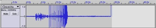
By using the tool magnifier we extend the needed part.
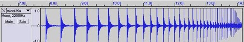
By menu View – Zoom we can get to the initial position. Click on the icon and place the cursor at the first impact. After clicking the number that corresponds to time appears in the left bottom corner. We round off the time to hundredths of seconds. By this method we can determine all times that are needed for plotting the desired graphs.
In Table 1 impact time t and times between impact and bounce for the first 11 impacts are summarized.
Results 1
| impact |
1 |
2 |
3 |
4 |
5 |
6 |
7 |
8 |
9 |
10 |
11 |
| t/s |
7.65 |
8.14 |
8.57 |
8.96 |
9.33 |
9.67 |
9.98 |
10.26 |
10.53 |
10.77 |
11.00 |
| t/s |
0.49 |
0.43 |
0.39 |
0.37 |
0.34 |
0.31 |
0.28 |
0.27 |
0.24 |
0.23 |
|
| v/ m/s |
2.403 |
2.109 |
1.913 |
1.815 |
1.668 |
1.521 |
1.373 |
1.324 |
1.177 |
1.128 |
|
| k |
0.88 |
0.91 |
0.95 |
0.92 |
0.91 |
0.90 |
0.96 |
0.89 |
0.96 |
average |
0.92 |
Table 1
Impact velocity is calculated using the equation for vertical motion: v = g Δt/2.
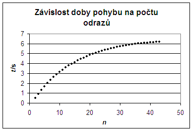
Figure 1: Time of motion dependence on numbers of bounces.
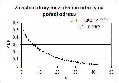
Figure 2: Dependence of times between two bounces on number of bounces.
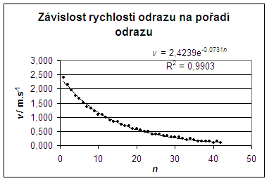
Figure3: Bounce velocity dependence on number of bounce.
Results 2
In Table 1 the coefficients of restitution were calculated for each two adjacent times and then its average value was determined. However, it is better to calculate this by using the regression function in Microsoft Excel. An exponential function v = 2.4239 · e-0.0731 n with the coefficient R2 = 0.9903 fits very well to our data. As the domain of the function is a subset of the natural numbers, it is a geometric sequence. The common ratio is our coefficient of restitution: \[k=\frac{v_{n-1}}{v_n} = e^{-0.0731} = 0.930 \]
A geometric sequence with common ratio e-0.0731 also corresponds to the dependence of time between two bounces on the number of bounces Δt = 0.4942·e–0.0731 n R2 = 0.9903. This geometric sequence is convergent; therefore the sum is given by: \[ s_n = \frac{a_1}{1-q} = \frac{0.4942\cdot e^{–0.0731}}{1-e^{–0.0731} } = 6.56\,\mathrm{s}.\]
The infinite sum corresponds to the whole time of motion of the ball.
Conclusions:
We can see from the plots that the velocity after every impact exponentially decreases. It follows the geometric sequence. The time between two bounces is a convergent geometric sequence with the same common ratio; the sum of the times is convergent.
Free fall of solids
Introduction
If we let fall some iron nuts tied together, they will causes sounds which can be recorded by microphone and computer. The distribution of nuts on the string affects the resulting sounds, mostly their regularity.
Guidelines:
Tools: Microphone with connector (jack) for connection with computer. computer. program AUDACITY. iron nuts (M10) on a string.
Tasks:
1) Measure using the microphone the impacts of nuts that are uniformly distributed on strings; next, increase the distances and measure again.
2) Make a plot of these experiments
Principle:
Tie six nuts on a string with a spacing of 25 cm. Hold the string in such a way that the bottom nut touches the surface. In the vicinity of this nut place the microphone. After stopping any motion of the string, let it fall down. To record the sounds and determine the needed times use the program AUDICITY (as was explained earlier). The newspaper has proved a good surface. The distance between the microphone and the nuts needs to be adjusted to get the best signal.
Next, tie the five nuts with the spacings:
10 cm – 30 cm – 50 cm – 70 cm
Then perform the free fall and find out the needed times.
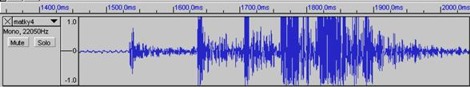
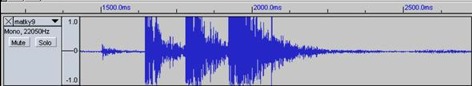
Results: Record of noise in program AUDICITY
Six nuts distributed with equidistance of 25 cm (5 impacts).
5 nuts distributed with increasing distances (4 impacts).
Table 1: The times of bounces_
| Number of impact |
t/s |
| 1 |
1.535 |
| 2 |
1.637 |
| 3 |
1.706 |
| 4 |
1.764 |
| 5 |
1.815 |
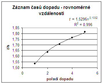
Figure 1: The time dependence of the sequence of bounces – the equidistance distribution.
Table 2
| Rank of impact |
t/s |
| 1 |
1.537 |
| 2 |
1.647 |
| 3 |
1.781 |
| 4 |
1.923 |
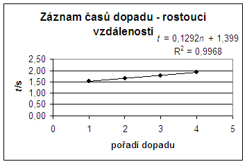
Figure 2: The time dependence of the sequence of bounces – increasing distances.
Conclusions: From Figure 1 it is obvious that free fall is an accelerated motion. Although the nuts are regularly distributed, every next nut falls down in a shorter time than the previous one.
Figure 2 shows that if the distances between nuts increases quadratically (10 cm, 40 cm, 90 cm, 160 cm) the times between impacts are the same, confirming that the free fall is a uniformly accelerated motion as given by s = 1/2 gt2.