About paper
Czech originalThe Propeller in Lab Exercises
A two-bladed propeller attached to the axis of a model DC motor can become a very useful tool to study many physical phenomena. It can be used in physics during lab or frontal work of students, and especially in a physics seminar. Here we present methodical instructions on four lab exercises with a propeller: (1) rotation, (2) propeller and monitor, (3) propeller flywheel, (4) pull of the propeller.
1) Rotation
(2nd year of grammar school or 7th class of elementary school)
Introduction
The propeller, when supplied with constant voltage, rotates very regularly with a very short period. The period can be changed by simply changing the voltage supply. Pupils measure the period of one revolution in relation to the voltage input to the motor. To observe such a fast motion the students will learn how to use a photoelectric sensor.
Methodical instructions
First it is necessary to demonstrate how a photoelectric sensor works. If the invisible infrared light beam is crossed, the computer registers a change on the graph from 1 to 0 and back. It is important to say, that we are using a two-blade propeller, therefore one revolution crosses the light beam twice.
Tasks:
1) Determine one period T of the propeller for voltage of 2V, 3V, 4V,...9V.
2) Draw a graph: Dependency of period T on voltage U and draw the correct curve.
3) Answer the following questions from the graph and the table:
a. How does the period of one revolution change when increasing the voltage to the motor?
b. Try to determine the period of one revolution, if the voltage is 6.5V.
c. What voltage needs to be supplied to the motor to make one period of revolution last 0.080 s?
Tools:propeller and motor with a handle, adjustable DC voltage source(up to 9V) with a built-in voltmeter, an ISES computer interface card, a photoelectric sensor.
We set the time of measurement to 0.5 s, sampling rate to 1000 Hz, manual start. After each measurement students determine the difference (delta) of the period T. They set the voltage in the range requested.
Here are typical results:
| U/V |
2 |
3 |
4 |
5 |
6 |
7 |
8 |
9 |
| T/s |
0.133 |
0.095 |
0.071 |
0.063 |
0.056 |
0.050 |
0.048 |
0.047 |
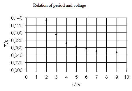
Conclusion
Pupils will learn to use a photoelectric sensor, create a graph with a spaced curve and to read the needed values from it. The lab exercise is a simple way to teach terms used in rotary motion, such as “Revolutions per given time”. A higher frequency can be observed by students on a monitor.
2) Propeller and monitor
(4-year grammar school – physics seminar)
Introduction
Students observe the monitor of a computer through a rotating propeller. At a certain frequency, the blades seem to stop, and the apparent number of blades can be changed with a change in frequency. It is up to the students to examine the relation between the number of stopped blades of the propeller and the frequency. They then try to explain the stroboscopic effect.
Methodic instructions
First it is necessary to show the students how such a phenomenon is created with the lowest possible frequency. By fine-tuning the voltage we create first an image with eight “stopped” blades. Then we insert the propeller into the photoelectric sensor and determine the period T.
Tasks
1) Examine the relation of the number of “stopped” blades of the propeller (in the order of 8, 6, 4 and 2) and the period of rotation T.
2) Measure the light emitted by the monitor using a photoresistor.
3) How do you explain the “stopped” blades?
Tools: propeller and motor with a handle, adjustable DC voltage source (up to 9V) with a built-in voltmeter, a photoresistor (e.g. WK 65075), an ISES computer interface card, a photoelectric sensor, an ohmmeter module.
We set the time of measurement to 0.5 s, sampling rate to 1000 Hz, manual start.
1) Students slowly raise the frequency until they get 8 blades, 6 blades, 4 blades, 2 blades. They ignore more-bladed images. Sometimes it may not be possible to achieve the 2-blade image. Here is a typical example of a measurement.
Dependency of period T on number of blades n
| n |
8 |
6 |
4 |
2 |
| T/ms |
129 |
95 |
69 |
35 |
| T/n/ms |
16,1 |
15,8 |
17,3 |
17,5 |
If they plot the results into a graph, they get an accurate enough linear dependence T = a·n.
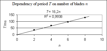
The constant a can be determined e.g. in Excel using a linear regression, or with any pair in the T/n table. The result of the regression is a = 16.2 ms. The constant a is obviously a time value.
2) In the ISES panel we swap the photoelectric sensor for a photoresistor, which is placed with the sensor side on the monitor and a measurement is performed. Here is a typical measured waveform:
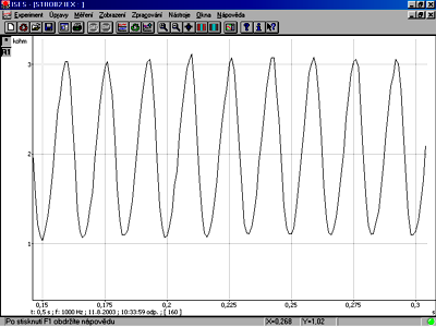
It is obvious that the brightness of the monitor oscillates periodically. From this graph the frequency of flashing is calculated
T0 = 17 ms.
3) The secret behind the “stopped blades” lies within the blinking of the monitor. The observed effect can, then, be explained as a stroboscopic phenomenon. Students surely observed this effect on television, e.g. with car wheel movements, which turn unrealistically slow, sometimes even backwards.
Our monitor had a refresh rate of 60 Hz (this value can be changed in Windows) and that means a period of T0 = 16.7 ms. This is a value which differs only by 3 % from the measured a. The constant a is therefore a period of flashing of the observed monitor.
If there are in the classroom more contemplative students who are, at the same time, very keen observers, we can perform a more thorough analysis of the experiment. When raising the frequency, the students may notice that the number of blades stopped is: 8, 6, 4, 6, 8, 2. This is quite a problematic task. Here is the solution:
The dark image of the propeller against the monitor is created when the blades cover the same place over and over again at the same time as the light from the monitor illuminates them. The number of stopped blades depends on the angle α, which the blade of a propeller travels during the period of flashing T0. For an angle measured in radians we can say that
\[ \tag{1} \alpha = \frac{2\pi}{T} T_0\]where T is the period of the propeller rotation.
2 blades can be seen when \( \alpha = \pi + k\pi, \) where kϵN0. When compared with equation (1), we get \( T = \frac{1}{k+1}\cdot 2T\).
4 blades can be seen when \( \alpha = \frac{\pi}{2} + k\pi. \) When compared with equation (1), we get \( T = \frac{2}{2k+1}\cdot 2T\).
6 blades can be seen when \( \alpha = \frac{\pi}{3} + k\pi\), \( T = \frac{3}{3k+1}\cdot 2T\) but also if \( \alpha = \frac{2\pi}{3} + k\pi\), \( T = \frac{3}{3k+2}\cdot 2T\).
8 blades can be seen when \( \alpha = \frac{\pi}{4} + k\pi\), \( T = \frac{4}{4k+1}\cdot 2T\) but also if \( \alpha = \frac{3\pi}{4} + k\pi\), \( T = \frac{4}{4k+3}\cdot 2T\).
A higher voltage means a shorter period T. The images will appear here in order from the longest period (fractions containing k = 0) to the shortest.
| Fraction |
4,00 |
3,00 |
2,00 |
1,50 |
1,33 |
1,00 |
| Number of blades |
8 |
6 |
4 |
6 |
8 |
2 |
| α |
45° |
60° |
90° |
120° |
135° |
180° |
This sequence does not depend on the refresh rate of the monitor.
In the concrete, for our 60 Hz frequency theory and experiment were pretty much equal:
| Number of blades |
8 |
6 |
4 |
6 |
8 |
2 |
| Ttheory/ms |
133 |
100 |
67 |
50 |
44 |
33 |
| Texper/ms |
129 |
95 |
69 |
53 |
45 |
35 |
To conclude, it must be said that we can see more than 8 blades, but this is hard to measure, as the image is unstable. With higher frequencies the “blade bending” effect can occur, which is most probably connected to the lines of the monitor.
Shorter periods than 35 ms were impossible to achieve with the motor used.
Conclusion
Students will become familiar with the stroboscopic effect, describe it mathematically and learn to use it to measure the refresh rate of a monitor. More broadly, they will learn to calculate an unknown frequency using a frequency standard, which is a common exercise in physics and metrology.
3) Flywheel propeller
(4-year grammar school – physics seminar)
Introduction
Students grab a spinning propeller by the handle and move it around. Doing this, they feel various forces. They are basically examining the gyroscopical effect, which is, as of yet, unfamiliar to them in theory and most likely in real life, too. It is, therefore, a discovery of something unknown – a heuristic experiment.
Methodical instructions
Task: When tilting the propeller, you feel various forces. Examine this phenomenon. Change the parameters of the experiment and note as many results of observation (no clarification needed).
Tools: Propeller and motor with handle, adjustable DC voltage source (up to 9V).
A rotating propeller is grabbed by the handle and placed in a vertical position. We tilt it downward and back again.
According to the impulse equation \(\vec{M} = \frac{\Delta\vec{b}}{\Delta t} \), where \( \vec{M} \) is the momentum of acting force and \( \vec{b} \) is the angular momentum.
This equation is then put into connection with the picture:
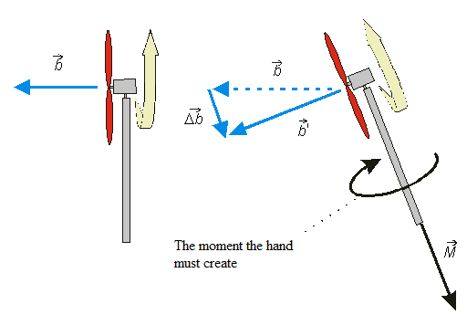
The most important thing is that the momentum of force \(\vec{M}\) must have the same direction as Δ\(\vec{b}\)!
The handle must be grabbed with the fingers so as to create torque in the indicated diretion. If the handle is gripped too softly, the handle will turn in the hand in the opposite direction than indicated.
It is obvious from the equation that the amount of torque depends on the change of angular momentum. Students should, through experimentation, discover that:
a) opposite momentum is needed to tilt upwards than to tilt downwards.
b) when changing the direction of twisting the propeller, the situation changes.
c) a bigger momentum is needed when the propeller rotation velocity is higher.
d) if the tilting is performed in a shorter time, more momentum is needed to hold the handle.
This experiment was performed in a physics seminar of the third year of a 4-year grammar school. In the seminar, girls almost totally outnumber boys, and all of them have chosen the seminar as a preparation for entrance exams for studying medicine. Here is an example of the observation results:
Group A
When turning the propeller in the direction of the turning of the propeller (away from us), we feel as if the propeller wanted to turn in the opposite direction by itself – “it resists”.
1) The larger the curve we draw with the propeller, the smaller the “propeller resistance” is
2) The slower the rotation, the smaller the “propeller resistance”.
3) The propeller resistance depends on the velocity with which we are turning the propeller. The faster we move, the larger the “propeller resistance”.
Group B
We connect the propeller so that the first turn points left. When moving the propeller upwards, we feel a tingling sensation on the lower side of our hand (against the motion), when moving downwards we feel the tingling sensation against the upper side of our hand.
We connect the propeller so that the first turn points right and observe the opposite effects.
Group C
1) The propeller actually cuts through air. If we move it in the direction in which it “cuts”, it is as if it tried to run away (when moving the propeller down, the blade part that cuts the air moves down).
2) When moving the propeller against the cutting direction, there is some resistance.
3) The propeller is affected by the air flow into the middle of the propeller when “waving” – it slows down.
Group D
We found out that when moving the propeller:
1) In an up-and-down motion:
· We feel the handle deflect to the sides
· Upward movement: The left side of the propeller lifts up
· Downward movement: The right side of the propeller lifts up
2) If the propeller is connected the other way (propeller spins in the other direction) – deflections are opposite to those in 1).
3) With a higher rotation frequency this movement is more perceptible.
The best description was probably given by group D. It is interesting to note that both students solve problems in exams flawlessly (they both have an A in the seminar) and here, they have proven a sense of experimentation and systematic work.
Conclusion
This task differs from the usual lab exercises; students examine a phenomenon, the theory of which they don’t know yet. The task is very useful in that the students uncover the law on their own, whereas in the majority of cases, the laws are described by the teacher. Moreover, students learn to formulate the results of their observation.
4) Pull of the propeller
(4-year grammar school – physics seminar)
Introduction
The pull of a propeller grows with the frequency of rotation. Higher frequencies, however, need a higher electric input of the motor. The relation between pull, frequency and electric input can be experimentally measured and the regression found in Excel.
Methodical instructions
If the students are unfamiliar with measuring frequency using a photoelectric sensor, they need to learn to do it, first.
Tasks: Examine how the pull depends on frequency, how frequency depends on input and how pull depends on input. Find the regressions.
Tools: propeller and motor with a handle, adjustable DC voltage source (up to 9V), an ISES computer interface card, a photoelectric sensor, an ohmmeter module, a stand with a pivot, a ruler, a tape measure, an ammeter, a voltmeter.
Students build an apparatus according to the picture. By adjusting the voltage they try to make the deviation xgrow by 1 cm each time. Each time, they have to measure the frequency of the propeller (using the photoelectric sensor), the current going into the motor and voltage at the motor. They measure a distance of l = 32.5 cm, the motor and propeller will be considered a point with a mass of 29 g. Students have a task of finding out how to calculate the pull of the propeller using the angle α.
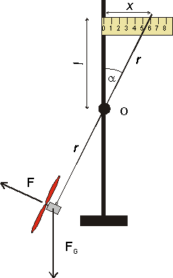
Derive the equation of force: If the motor doesn’t revolve around the pivot O, the momentums are equal: \[ F \cdot r = F_G \cdot r \cdot \sin \alpha, \] \[ F = F_G \cdot \sin \alpha, \] \[ F \cdot r = mg \frac{x}{\sqrt{x^2 + l^2}}. \]
The following table sums up all the data needed to create the graphs.
| f/Hz |
x/cm |
F/N |
U/V |
I/A |
P/W |
| 11.2 |
1.0 |
0.009 |
2.02 |
0.11 |
0.222 |
| 15.0 |
2.0 |
0.017 |
2.68 |
0.15 |
0.402 |
| 18.0 |
3.0 |
0.026 |
3.67 |
0.19 |
0.697 |
| 20.6 |
4.0 |
0.035 |
4.46 |
0.23 |
1.026 |
| 22.9 |
5.0 |
0.043 |
5.19 |
0.27 |
1.401 |
| 24.7 |
6.0 |
0.052 |
6.01 |
0.30 |
1.803 |
| 26.5 |
7.0 |
0.060 |
6.87 |
0.35 |
2.405 |
| 28.8 |
8.0 |
0.068 |
7.82 |
0.40 |
3.128 |
| 30.0 |
9.0 |
0.076 |
8.55 |
0.42 |
3.591 |
| 31.0 |
10.0 |
0.084 |
9.39 |
0.44 |
4.132 |
The graphs can easily be created in Excel.
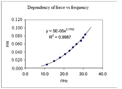
The force is proportional to the square of frequency.
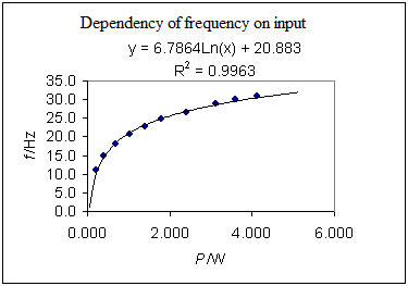
At first, frequency rises quickly with growing electrical input. At a higher electrical input,this growth slows down. The logarithmic function describes this behaviour best.
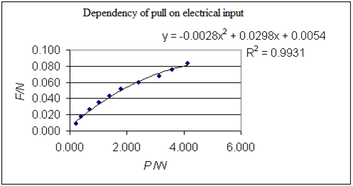
In the measured range the concave graph is best represented by a second degree polynomial
Conclusion
Students measure a complex laboratory experiment combining mechanics and electricity. The measured values are, again, heuristic, because the dependencies listed herein aren’t taught in physics classes at grammar schools. Students search for a mathematical description of the measured results.