About paper
Czech originalModern Photometry – Using a Phototransistor And a Multimeter
Perceiving light is the first (and maybe even the last) sensation in a person’s life and light is therefore so tightly connected to life that every cult or religion places some value on it. Even Genesis mentions the light: “And God said, “Let there be light,” and there was light. And God saw that the light was good. And God separated the light from the darkness.” [1]
For physics, the study of light and energy transfer through radiation is a very important field; here the borders between classical and quantum physics – we warded off the ultraviolet catastrophe using packets of hf energy (Max Planck), Einstein’s special relativity theory solved the independence of light-speed on the frame of reference. At school it is difficult to measure light-speed or determine spectral density of light. What is possible, however, is:
- Create a photometry lab experiment,
- Use Excel to draw polar graphs,
- Measure the output of a light-bulb,
- Measure the quantum light emission efficiency on a PN junction,
- Create a lab experiment on light polarisation and laser,
- Draw an Excel graph in polar coordinates.
Our first tool will be a photometric probe.
The probe is made from a phototransistor BPW42 (made by Vishay-Telefunken). It is a silicon phototransistor with maximum voltage Uke = 30 V and maximum connector current of 50 mA. The saturation voltage is approx. 400 mV and the collector’s current without illumination is lower than 200 nA. The probe connects very simply, as follows:
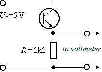
Fig. 1: The connection of the probe
The connector current grows linearly with illumination and we can measure voltage from 0.01 V to 4.5 V on the resistor. In this range the output voltage is directly proportional to illumination. To calibrate, it is good to use a 60 W matte light-bulb and a luxmeter, e.g. PU150 METRA. This phototransistor is most spectrally sensitive to the 830 nm (infrared light) wavelength, and if we calibrate the device using daylight and use a light-bulb to measure, the measurement will be hindered by a systematic error. The construction of the probe is not complicated, a felt-tip pen plastic tube will do fine (e.g. Centropen 0.3 liner 2921, or something similar), just drill the tip to be just the transistor diameter.
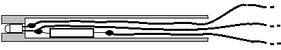
Fig. 2: The probe
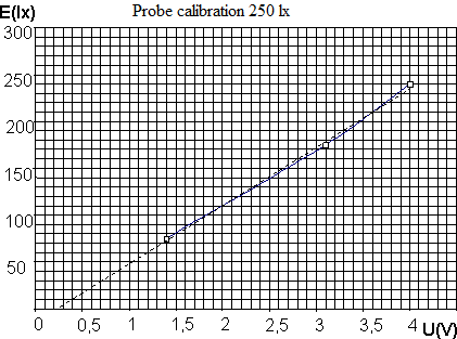
Thanks to the good linearity of our probe, it is only required to measure the output voltage for E = 0 lx, then increase the illumination until the output of the probe shows 4 V and then we use the lux meter to measure the E maxillumination. Measured illuminations in the given range can be read from a graph, but while making the graph on a computer the option presents itself to calculate a linear approximation from the graph. For the used probe (grey casing), Ex = 63.47 (Ux − 0.25). We measure the illumination E at relatively small distance and the probe with range up to 250 lx is suited for use with small-input light-bulbs.
To measure higher illuminations we only need to use a smaller resistance resistor – another probe has a resistor with R = 470Ω and it is usable for measurements of up to 1100 lx (red casing). The illumination calculation linear approximation is Ex = 226.8 (Ux – 0.15)
Obr. 3
Another tool is a modified roll film development tank.
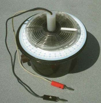
Fig. 4
We add a protractor to the lid of our tank. Two plastic protractors glued to the lid will do. The tank coil has two parts, the lower of which we are going to use. We place a cylindrical tube inside, glue an E 10 light-bulb socket inside and get the wires outside of our tank. We glue a protractor needle/arrow on the face of the tank. We close the tank and place a portion of the coil with the light-bulb inside from above. We measure the distance of the light-bulb and the tank bottom and drill a hole in the same height. There we place our phototransistor probe.
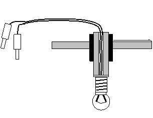
Fig. 5: Part of the coil with the light-bulb
We divide the 360° of the circle into 72 angles and measure the illumination for each one (one part has 5°). We read the values on our digital multimeter and in Excel, we calculate the illumination levels using our calibration graph.
In Excel, it is easy to create a polar graph of luminosity:
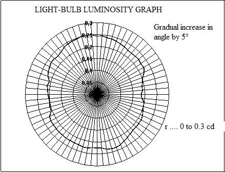
Fig. 6
It is obvious, that the light-bulb doesn’t illuminate all angles equally. The two opposing maximums are the directions perpendicular to the wire plane, which is in the used type of light-bulb stretched to resemble the upside-down turned letter V. The lowermost values are in the directions parallel to the plane of the wire and they are created by the fact that the wire further away is shaded by the one that’s closer to our probe. The difference in illumination achieved is approximately 60 lux, but this is imperceptible by the naked eye. The average illumination is approximately 210 lx, and knowing this we can calculate the average illumination, luminous flux and specific light output of the light-bulb.
Average illumination equation: \[ L = Er^2 = 210 \cdot 0.32^2 \,\mathrm{cd} = 0.215\,\mathrm{cd}.\]
To calculate the total luminous flux of the light-bulb, we presume that the light-bulb wire shines equally into all directions and we ignore the loss of luminous flux aimed into the lamp cap. \[ \Phi = 4\pi L = 12.56\cdot 0.215\,\mathrm{lm} = 2.7\,\mathrm{lm}.\]
To calculate the specific light output of the light-bulb, we divide the total luminous flux by electrical input (we also need to know the current going through the light-bulb, in our case I = 52 mA): \[ \frac{\Phi}{P} = \frac{\Phi}{UI} = \frac{2.7}{6.3\cdot0.052} \,\mathrm{\frac{lm}{W}} = 8.24 \,\mathrm{\frac{lm}{W}} \]
In technical literature [2] one can find values of 6 to 8 lm×W-1 for a light-bulb with tungsten wire.
The polar graph for a red LED has a significant directional character:
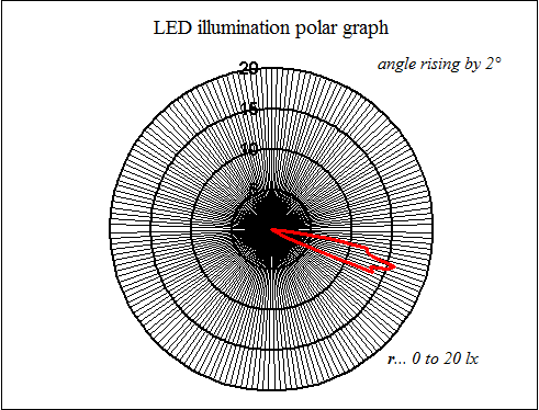
Fig. 7
Here, the option to determine the quantum efficiency as a ratio of number of emitted photons per second and number of electrons that passed through the LED’s PN junction. The number of electrons per second is: \[ n_e = \frac{I_D}{q_e} = \frac{15.9\cdot10^{-3}\,\mathrm{A\,s^{-1}}}{1.602\cdot10^{-19}\,\mathrm{A}} = 9.92\cdot10^{16}\,\mathrm{s^{-1}},\]
ID is the current flowing through the diode.
The number of photons emitted by the diode per second is the quotient of radiant flux P and the energy of one photon. The luminous flux P equals to ϕ / 683 for the wavelength of 660 nm. The luminous flux itself will be determined as ΔΦ = ΔΩ l(α), \[ \Delta \Phi = \Delta \Omega \frac{E(\alpha)}{r^2}, \]
Ω is the space angle in steradians, E(α) is the illumination measured at the distance of r = 3 cm. The angle α = 0 is for the maximum luminous intensity. The space angle addition equation to calculate ΔΩ is obvious from the picture:
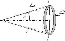
Fig. 8
The equation is as follows: \(\Delta S = r \Delta \alpha 2\pi r \sin \alpha \); from this we can conclude that \( \Delta \Omega = \frac{\Delta S}{r^2} = 2\pi \sin \alpha\, \Delta \alpha. \)
The value Δα needs to be in radians.
| α ° |
E (lx) |
ΔΩ (sr) |
ΔΦ (lm) |
| 1 |
15.5 |
0.9569 ·10-3 |
13.35 ·10-3 |
| 2 |
15.11 |
1.9136 |
26.00 |
| 3 |
13.98 |
2.8696 |
36.11 |
| 4 |
13.22 |
3.8248 |
45.50 |
| 5 |
13.60 |
4.7788 |
58.49 |
| 6 |
13.60 |
5.7314 |
70.16 |
| 7 |
11.42 |
6.6822 |
68.68 |
| 8 |
7.86 |
7.6310 |
53.98 |
| 9 |
5.44 |
8.5775 |
41.99 |
| 10 |
3.38 |
9.5213 |
28.96 |
| 11 |
1.18 |
10.4622 |
11.12 |
|
|
|
total Φ = 454.34·10-3 lm |
Radiant flux \[ P = \frac{\Phi}{683}\cdot\frac{555}{660}=\frac{0.454}{683}\cdot\frac{555}{660} = 0.559\,\mathrm{mW}.\]
The number of photons emitted per second \[ n_f = \frac{P}{hf} = \frac{P}{h\frac{c}{\lambda}} = \frac{0.559\cdot10^{-3}}{6.626\cdot10^{-34}\frac{3\cdot10^{8}}{0.66\cdot10^{-6}}}\,\mathrm{s^{-1}} = 1.856\cdot10^{15}\,\mathrm{s^{-1}}.\]
The quantum efficiency \(\eta = \frac{n_f}{n_e} = \frac{1.856\cdot10^{15}}{9.92\cdot10^{16}} = 0.0187 = 1.87\,\% \).
On average, one hundred electrons are needed to create 2 photons, and this ratio is very low. On the PN junction itself, the quantum efficiency is higher, but the diode material – air transition causes total internal reflection and photons are absorbed by the diode material (epoxy, gallium arsenide, gallium phosphide, etc.).
To study polarized light a third tool was created – the polarizer.
We replaced the polarizing film in the angled holder with a mobile phone display. The display itself is rather complicated (see fig. 9).
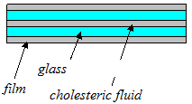
Fig. 9
On its way through the polarizer film the light polarizes, in the cholesteric fluid its polarization plane turns 90° and passes through the other foil, whose polarization plane is turned 90° as well. This can be proven with a simple experiment: we observe light reflected from the shiny paint of a school desk or the reflection from a whiteboard and set the filter to minimize the amount of light passing through. Then we turn the polarizer 180° along the vertical axis – the gleam shines perfectly.
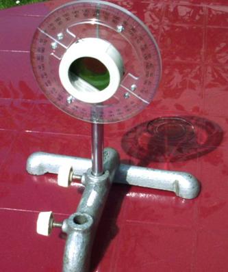
Fig. 10
The light of a light-bulb is non-polarized and to measure it we use one filter as a polarizer and another one as an analyzer. We perform the measuring using the set-up in figure 11.
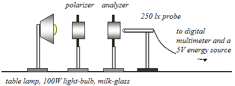
Fig. 11
It is good to power the light-bulb from a DC source, otherwise the measurements oscillate – the light-bulb wire powered with AC has no constant temperature.
A polar graph showing the relation of illumination and analyzer angle shows two maximums and two minimums of 70 and 40 lx, respectively. We observe a much greater difference with the naked eye and this is important to explain.
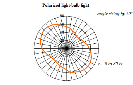
Fig. 12
The polarization film is usable in a limited wavelength range, e.g. the BK27 film is effective in the 320 to 700 nm range – see [4]. Infrared light passes through both filters without polarization and the probe sees them in full intensity.
The last measurement suggestion is the study of laser light. We will use one filter, a probe and a laser pointer:
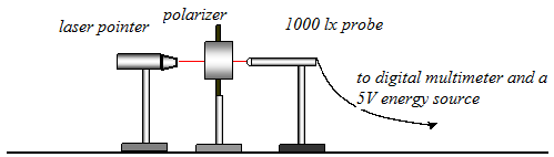
Fig. 13
The relation of the probe illumination and the angle of the polarizer is very distinct:
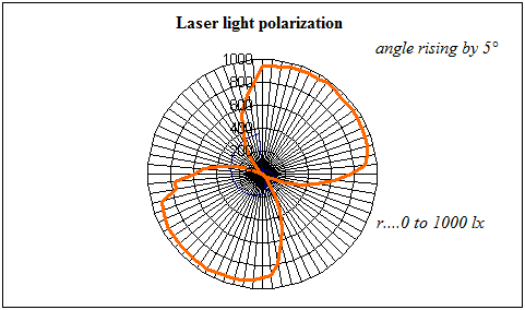
Fig. 14
The graph has two minimums and two maximums of up to 1000 lx. The reason is that laser light is already polarized during its creation and its wavelength falls into the effective range of the polarizer film.
Experiments suggested above are not time-consuming and all students can do them with their knowledge of IT sciences. The unusual polar graphs are aesthetically appealing and present a different point of view than the typical Cartesian graph. An important moment during these experiments is also the introduction to the working principles of a phototransistor, an LED and a diode laser: here I can recommend, apart from secondary school textbooks, the work of our Slovakian colleagues Fyzikálne základy elektroniky, wherein the authors explain everything one can encounter in electronics in an easily accessible manner [3].
References:
[1] Bible, English Standard Version, Genesis 1:3-4
[2] Miškařík, S.: Moderní zdroje světla, SNTL 1979 (in Czech)
[3] Baník Ivan, BaníkRatislav, Baník Igor: Fyzika Fyzikálne základy elektroniky, Slovenská technická univerzita v Bratislavě 1999 (in Slovakian)